
“What are good measurements and good error analysis? High likelihood that the ‘true’ value is within your given uncertainty, while keeping the uncertainty as small as possible.” – Professor Mark Battle
The following discussion of uncertainty is largely taken from the book, An Introduction to Error Analysis, by John R. Taylor.
Experience has shown that no measurement, however carefully made, can be completely free of uncertainties. Scientists refer to this uncertainty as “experimental error”, but the word “error” here does not have the usual meaning of “mistake” or “blunder”. Because the whole structure and application of science depends on measurements, the ability to evaluate these uncertainties and keep them to a minimum is crucially important!
You should be aware of some types of uncertainties to which almost any measurement is subject:
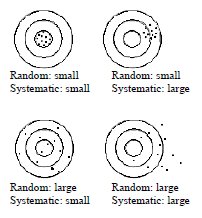
Random and systematic errors in target practice. (From “An Introduction to Error Analysis” by John R. Taylor.)
- Instrumental Resolution – reflects the fineness of the divisions on the measuring device. For example, one millimeter is the smallest division on a typical meter stick. You can probably estimate between divisions to \(1/4\) or \(1/2\) mm. Another example would be a voltmeter that the manufacturer states is only accurate to \(\pm 0.001\) V.
- Random Error or Inherent Uncertainty – experimental uncertainty that can be revealed by repeating the measurement. For a set of repeated measurements, the “most representative” value is given by the average or mean, \(\bar{x}\). The precision of the mean reflects the random variation from measurement to measurement (i.e. how tight the measurement values are around the average) quantified by the standard error of the mean, \(S_{m}\).
- Systematic Error – an estimate of a measurement’s accuracy, due to measurement or equipment problems, which cannot be revealed by repeating the measurement. By “systematic” we mean something that affects each measurement in a non-random way. So, if the bottom \(1\) cm of your meter stick is missing (and you don’t notice!), all your lengths will be \(1\) cm too long. More generally, systematic error represents the difference between your measured value and that which would be obtained by the mythical “perfect experimenter”, using “perfect” measurement instruments. The tricky part about systematic errors is that you usually don’t know they’re there, so they’re hard to estimate!
Reporting Measurements: Best Estimates \(\pm\) Uncertainty
In general, the result of any measurement of a quantity \(x\) is stated as
$$(\rm{measured}\:x) = x_{\rm{best}} \pm \delta x.\label{1}\tag{1} $$
This statement means that your best estimate of the quantity concerned is \(x_{\rm{best}}\), and you’re reasonably sure the value lies somewhere between \(x_{\rm{best}}-\delta x\) and \(x_{\rm{best}}+\delta x\). The number \(\delta x\) is called the uncertainty or error in the measurement of \(x\). For convenience, the uncertainty \(\delta x\) is always defined to be positive, so that \(x_{\rm{best}}+\delta x\) is always the highest probable value of the measured quantity and \(x_{\rm{best}}-\delta x\) is the lowest. In our labs, and experimental science in general, the uncertainty of a measurement, \(\delta x\), is a function of the number of times that the measurement is made:
- For single measurements, we measure some quantity, \(x\), to the best of our ability, and then make a judgment of its uncertainty, based primarily on the resolution of the instruments used.
- A simple example would be measuring the length of, say, a Twinkie with a ruler marked in mm. If your best estimate is \(68.5\) mm and you’re pretty sure that the value is between \(68.0\) and \(69.0\) mm, then you would report the length as
$$ \rm{Twinkie\:length}=68.5\pm 0.5\:\rm{mm}.$$
- A simple example would be measuring the length of, say, a Twinkie with a ruler marked in mm. If your best estimate is \(68.5\) mm and you’re pretty sure that the value is between \(68.0\) and \(69.0\) mm, then you would report the length as
- Where repeated measurements are taken, one can use statistical analysis to state \(x_{\rm{best}}\) and its uncertainty. The \(x_{\rm{best}}\) is generally given by the mean or average, \(\bar{x}\), of the data set, and its uncertainty by the “standard error of the mean”, \(S_{m}\). The beauty of repeated measurements is that you can ignore the uncertainty of each individual data point. Note: If you’re more interested in the range of the result (i.e for plotting error bars) than its precision, then the standard deviation, \(s\), may be a better estimate of the uncertainty.
Statistical Analysis of Random Uncertainties
One of the best ways to assess the reliability of a measurement is to repeat it several times and examine the different values obtained. Statistics is a very useful tool for analyzing measurements and estimating error in a “large” set (at least \(5\), and preferably more) of repeated measurements.
Suppose we have \(N\) measurements of some quantity, \(x_{1}\),\(x_{2}\),\(\ldots\),\(x_{N}\). If there is no systematic error in a set of measurements, the mean (or average) is the best approximation to the “true” value that we can obtain from a set of measured values:
$$\bar{x} = \sum^{N}_{i=1}\frac{x_{i}}{N}.\tag{2}$$
The standard deviation is technically the root-mean-square average deviation of the data from the average value. It is a measure of the typical variability from measurement to measurement, and says that if your measurements are distributed on a “normal” or “bell-shaped” curve, then \(68\%\) of your data points will fall within one \(s\) on either side of the mean value. The (sample) standard deviation is:
$$s = \sqrt{\sum^{N}_{i=1}\frac{(x_{i}-\bar{x})^{2}}{N-1}}. \tag{3}$$
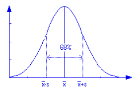
A sketch of a “normal distribution”, showing \(68\%\) of the data within one standard deviation of the mean.
The standard error of the mean is an estimate of the uncertainty in the mean, in the sense of roughly how far it may be from the “true” value. It is this quantity that answers the question, “If I repeat the entire series of \(N\) measurements and get a second mean, when do I have a \(68\%\) confidence that this second average will come close to the first one?”. The answer is that you should expect a second average (that results from redoing the set of measurements) to have a \(68\%\) probability of lying within one standard error of the first average that you determined. Thus the standard error of the mean is sometimes referred to as the \(68\%\) confidence interval. The standard error of the mean is:
$$S_{m} = \frac{s}{\sqrt{N}}. \tag{4}$$
How do we determine the number of measurements to take? As we make more measurements, \(N\) increases, and at first \(\bar{x}\) bounces around a bit, but the larger \(N\), the less \(\bar{x}\) changes. Similarly, \(s\) varies at first, but settles down to some value. However, \(S_{m}\) varies as \(1/\sqrt{N}\). Thus it gets smaller as \(N\) increases. Qualitatively, this says “the more numbers you average, the better the mean value is determined”. In reporting a result we usually want a “best” (mean or average) value and an estimate of its uncertainty. We report these as \(\bar{x}\pm S_{m}\). We will sometimes call \(S_{m}\) the precision of \(\bar{x}\). Note that \(S_{m}\) and \(s\) have the same units as the original measured values.
Significant Figures
See the discussion here as well.
Significant figures are also called significant digits. Because \(\delta x\) is an uncertainty, it should not be stated with too much precision. For example, it would be ridiculous to state the above measurement as
$$ \rm{Twinkie\:length}=68.5\pm 0.4764267\:\rm{mm}.$$
This leads to the following rule for stating uncertainties:
Experimental uncertainties should almost always be rounded to one significant figure.
One exception: If the leading significant figure in the uncertainty \(\delta x\) is a \(1\), then keeping \(2\) significant figures in \(\delta x\) may be better. For example, if some calculation gave the uncertainty \(\delta x = 0.14\), then rounding to \(0.1\) would be a substantial proportional reduction, so retaining the \(2\) figures, \(0.14\), would arguably be better.
Once the uncertainty has been estimated, it determines the number of significant figures in the measured value through the following rule:
The last significant digit in any stated result should be of the same order of magnitude (in the same decimal position) as the uncertainty:
- \(98.\underline{26}\pm 0.\underline{03}\) mm
- \(30.\underline{0004}\pm 0.\underline{0002}\) g
- \(1\underline{30}\pm \underline{20}\) s
- \(5\underline{50,000}\pm \underline{10,000}\) people
In the Twinkie example, if you reported
$$ \rm{Twinkie\:length}=68.52443\pm 0.5\:\rm{mm}$$
the last \(4\) digits in the decimal part would be meaningless.
Absolute and Fractional Errors
Errors are either reported as absolute errors or as relative errors:
- The absolute error of a quantity has the same units as the measured value, and is simply what you report when you say you can only measure something to such and such certainty. From the Twinkie example, our absolute error is \(0.5\) mm. The absolute error is usually denoted with a small Greek delta, so for a quantity denoted by \(x\) (or \(y\), etc.) the absolute error would be written as \(\delta x\) (or \(\delta y\), etc.) as in Equation (\ref{1}). Absolute error must be used when graphing error bars (to know the size of the error bar) and when comparing one measured quantity to another.
- The relative error or fractional error of a quantity \(x\) is simply what fraction the absolute error is of the quantity itself, so
$$ \rm{relative\:error} = \frac{\rm{absolute\:error}}{\rm{best\:value}}=\frac{\delta x}{x}. (\rm{No\:units!\:They\:cancel!})\label{5}\hskip{5em}\tag{5}$$
The relative error is usually expressed as a percentage (by multiplying by \(100\%\)). So, for our Twinkie length measurement we have a relative error of \(0.5\:\rm{mm}/68.5\:\rm{mm})=0.007=0.7\%\). Note that if you have the relative error of a quantity, you can easily calculate its absolute error by rearranging the above equation.
Comparison of Two Measured Numbers
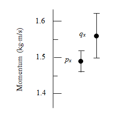
A Graphical Comparison of Measured X-Components of Momentum
Many experiments involve measuring two numbers that theory predicts should be equal. For example, the law of conservation of momentum states that the total momentum of an isolated system is constant. To test it we might perform an experiment with \(2\) carts that collide on a frictionless track (as we did in Lab \(2\) of \(\underline{\rm{Physics}\:1130}\)). Let’s say we measure the total momentum of the \(2\) carts before (\(\vec{p}\)) and after (\(\vec{q}\)) the collision and check whether \(\vec{p}=\vec{q}\) within experimental uncertainties. Suppose we measure
$$ \rm{initial\:momentum}\:\vec{p} = 1.49\pm 0.03\:\rm{kg\:m/s}\:\hat{x}$$
and
$$ \rm{final\:momentum}\:\vec{q} = 1.56\pm 0.06\:\rm{kg\:m/s}\:\hat{x}.$$
Here, the likely range for the x-component \(p_x\) (\(1.46\) to \(1.52\) kg m/s) overlaps the likely range for the x-component \(q_x\) (\(1.50\) to \(1.62\) kg m/s). Therefore, these measurements are consistent with conservation of momentum: they are equal within experimental uncertainties.
If, on the other hand, the two probable ranges were not even close to overlapping, the measurements would be inconsistent with conservation of momentum. We would have to check for mistakes in our measurements and calculations, look for possible systematic errors, and investigate the possibility that external forces (such as gravity and friction) are causing the momentum of the system to change.
Propagating Errors in Calculations
(When Two or More Uncertain Quantities are Combined)
Let’s continue now with error analysis. We often carry out calculations using measured values, and we must take into consideration the associated uncertainties since the result cannot be better than the data on which it was based.
- Uncertainty in Sums and Differences: Suppose that \(x\), \(y\), \(\ldots w\) are measured with uncertainties \(\delta x, \delta y, \ldots \delta w\) and we use the measured values to compute
$$ q = x + \ldots + z – (u+\ldots + w).$$
If the uncertainties in \(x, y,\ldots w\) are known to be independent and random, then the uncertainty in \(q\) is:
$$\delta q = \sqrt{(\delta x)^{2}+\ldots + (\delta z)^{2} + (\delta u)^{2} + \ldots +(\delta w)^{2}}.\label{6}\hskip{2.5em}\tag{6}$$
This is called a quadratic sum. Notice that even for the subtracted values, the estimate of the error in the result, \(\delta q\), adds the squares of the absolute error of each value (\(\delta x\) through \(\delta w\)) and then takes the square root of the total. - Uncertainties in Products and Quotients: Suppose that \(x,y,\ldots w\) are measured with uncertainties \(\delta x, \delta y,\ldots \delta w\) and we use the measured values to compute
$$q = \frac{x\times\ldots\times z}{u\times\ldots\times w}.$$
If the uncertainties in \(x, y, \ldots w\) are known to be independent and random, then the relative uncertainty in \(q\) is:
$$\frac{\delta q}{q} = \sqrt{\left(\frac{\delta x}{x}\right)^{2}+\ldots + \left(\frac{\delta z}{z}\right)^{2} + \left(\frac{\delta u}{u}\right)^{2}+\ldots + \left(\frac{\delta w}{w}\right)^{2}}.\label{7}\hskip{5em}\tag{7}$$
This is a quadratic sum of the relative errors of multiplied and divided values. If a particular form is not specified, you can report your calculated \(q\) with either relative error (usually given as \(\%\)) or absolute error (the relative error \(\times q\), with units), but make sure it is clear which one you are reporting. Remember: When dealing with the product or quotient of uncertain quantities, use the relative errors, and when we have the sum or difference of uncertain quantities, use the absolute errors themselves. See Equations (\ref{6}) and (\ref{7}). Easier examples for (\ref{6}) and (\ref{7}), using values with their respective uncertainties: \(a\pm\delta a\), \(b\pm\delta b\), and \(c\pm\delta c\):- What is the uncertainty of \(q = a + b + c\)?
$$\rm{Using\:Eq.\:\ref{6}:\:} \delta q = \sqrt{(\delta a)^{2}+(\delta b)^{2}+(\delta c)^{2}}.$$ - What is the uncertainty of \(q = \frac{a b}{c}\)?
$$\rm{Using\:Eq.\:\ref{7}:\:} \frac{\delta q}{q} = \sqrt{\left(\frac{\delta a}{a}\right)^{2}+\left(\frac{\delta b}{b}\right)^{2}+\left(\frac{\delta c}{c}\right)^{2}}.$$
- What is the uncertainty of \(q = a + b + c\)?
- Uncertainty in a Power: If \(x\) is measured with uncertainty \(\delta x\) and is used to calculate, say, \(q=x^{3}\), then we could write that as \(q=x\cdot x\cdot x\). However, the three \(x\) values here are the same quantity, so we know they are not independent. This requires a different combination of the errors; instead of the quadratic sum (as in Eq. (\ref{7}) above), we take a regular sum to allow for the largest possible error. Thus the relative error is given by
$$\frac{\delta q}{q} = \frac{\delta x}{x}+\frac{\delta x}{x}+\frac{\delta x}{x}=3\frac{\delta x}{x}.$$
This is true for any power, so for the equation \(q = x^{n}\) (where \(n\) is a fixed, known number), the fractional uncertainty in \(q\) is \(|n|\) times that in \(x\):
$$\frac{\delta q}{q}=|n|\frac{\delta x}{x}.\label{8}\tag{8}$$
For example, if you measure an area \(x\) as \(81\pm 6\:\rm{cm}^{2}\), what should you report for \(q=\sqrt{x}\) (square root of \(x\)), with its uncertainty? Answer:
$$q = x^{1/2} = (81\:\rm{cm}^2)^{1/2}=9\:cm,$$
$$\frac{\delta q}{q} = |n|\frac{\delta x}{x} = |\frac{1}{2}|\frac{\delta x}{x} = |\frac{1}{2}|\frac{6\:\rm{cm}}{81\:\rm{cm}}=0.037, $$
$$\rm{So},\:\delta q = 0.037 q = 0.037\times 9\:\rm{cm}=0.33\:\rm{cm} ,$$
$$\rm{and\:we\:report}\:q=\sqrt{x}=9.0\pm0.3\:\rm{cm},$$
where the error has been rounded to \(1\) significant figure, and the answer is reported with the same decimal places as the error.
For those of you comfortable with calculus, and who like knowing general rules (the sign of a good physicist!), the above three “rules” are all derived from one general formula for error propagation. For a function \(q\) of measured variables \(x, y,\ldots z\) the uncertainty in \(q\) is
$$\delta q = \left[\left(\frac{\partial q}{\partial x}\delta x\right)^{2}+\ldots +\left(\frac{\partial q}{\partial z}\delta z\right)^{2}\right]^{1/2} .$$
Let’s go back to significant figures for a minute. In a lab setting, significant figures are best given by the uncertainty of your measurements – the two rules from the significant figures section. But when uncertainty analysis is not required, use the following rules for combining values with differing significant figures:
- Multiplying/Dividing: A result should have the same number of significant figures as its least-significant-figure component. This is simple and makes sense if you think about the fact that a result can be no more precise than its least precise component.
- Adding/Subtracting: The decimal place precision is the key here – give your answer to the number of decimal places of the value with the least number of decimal places.
Two examples:
- Subtract \(0.52\) cm (\(2\) decimal places, \(2\) significant figures) from \(12.3\) cm (\(1\) decimal place, \(3\) significant figures). Answer: \(11.8\) cm (\(1\) decimal place, \(3\) significant figures)
- Here, we’ll check to see if the informal rules above are consistent with formal error propagation. Say you know the distance to your grandmother’s house is \(1237\pm 5\) miles [or use \((1.237\pm 0.005)\times 10^{3}\) miles, in scientific notation]. This has \(4\) significant digits. You estimate that the cost to drive your car is \(17\pm 3\) cents/mile (or \(0.17\pm 0.03\) dollars/mile). This has \(2\) significant digits. So, let’s evaluate the total cost of the trip to your grandmother’s house, first ignoring the uncertainties:
$$\rm{Total\:cost} = \rm{distance}\times\rm{cost/distance},$$
$$\rm{Total\:cost} = 1.237\times 10^{3}\:\rm{miles}\times 0.17\:\rm{dollars/mile},$$
$$\rm{Total\:cost} = 210.29\:\rm{dollars},$$
$$\rm{Total\:cost} = 210 (\rm{or}\:2.1\times 10^{2})\:\rm{dollars}.\:\:(2\:\rm{significant\:figures})$$
Now, let’s check what the propagation of errors says about significant digits. The “least-significant-digit” cost/mile estimate is only good to \(3\) parts in \(17\) relative error, (or \(3/17\times 100\%=18\%\)). So really the relative error of the result can be no better. Equation \((\ref{7})\) tells us that
$$\frac{\delta\rm{Total}}{\rm{Total}}=\sqrt{\left(\frac{\delta\rm{distance}}{\rm{distance}}\right)^{2}+\left(\frac{\delta\rm{Cost/mile}}{\rm{Cost/mile}}\right)^{2}},$$
$$\frac{\delta\rm{Total}}{\rm{Total}}=\sqrt{\left(\frac{5}{1237}\right)^{2}+\left(\frac{3}{17}\right)^{2}},$$
$$\frac{\delta\rm{Total}}{\rm{Total}}=0.18,$$
which is also \(18\%\). Why? Because the \(5/1237\) fraction is negligible compared to the larger \(3/17\) value. The absolute error in total cost, found by rearranging Eq. (\(\ref{5}\)), is \(\delta\rm{Total}=0.18\times 210.29\:\rm{dollars}=$37.85\rightarrow$40\) when rounded to one significant digit. This is why it makes sense to state the total cost as just \($210\), since you don’t know it any better than \($40\) either way.
![]()
