Building the Circuit

• Make sure that your UCS-30 is turned off before you start connecting cables to it.
• Connect a special high voltage cable from the positive HV output on the back of the UCS-30 to the HV input on the end of the detector.
• Attach a multi-pin pre-amp cable from the UCS-30 to the end of the detector.
• Use a standard BNC cable to connect the output of the detector to the input on the UCS-30.
• Use the USB cable to connect the UCS-30 to your computer.
• Connect the power cord for the UCS-30 and plug it in.
• Don’t turn on the UCS-30 until your instructor has had a chance to check your wiring.

Indicator Lights and Software Setup

• When the UCS-30 is turned on the positive HV light should be green.
• Open the USX software.
• Select Mode-PHA-Amp In from the menu bar.
• The High Voltage box in the upper left-hand corner is designed to take a number in volts. Figure out what to enter by looking at the HV value given on the hand-written sticker on the detector or cradle. It is different for each detector, but is around \(1000\:\rm{V}\). The voltages of the pulses corresponding to detections are very sensitive to the high voltage supply value, so once you have adjusted this setting do not change it during the lab.
• Set the amplifier’s coarse gain to \(2\) and the fine gain to \(1.00\).
• Now turn the HV on by clicking the button next to the voltage that you entered.
• If the software produces a warning here, stop and talk to your instructor.
• The positive HV light on the UCS-30 should turn red indicating that potentially dangerous high voltage is present. The activity light should also flicker red, indicating that the UCS-30 is receiving data.
• Click the green diamond Start Counts button in the upper left-hand corner to start acquiring data. The acquire light on the the UCS-30 should now be red.

You should begin to see data accumulate on the screen. The voltage of each pulse coming from the detector is measured by the MCA in the UCS-30, and the USX program plots the number of pulses received in each voltage “bin” (channel). Since the voltage of a pulse is proportional to the energy, the horizontal scale represents the energy, and the vertical scale records the number of gamma rays with that energy. Thus, the plot gives the energy spectrum of the gamma rays detected. (Note: since the horizontal scale has not yet been calibrated, the values do not represent the actual energy values.  You will be calibrating the scale later.)

Vertical Scale Notes

• You can switch between a logarithmic and a linear vertical scale using the Y LOG and Y Lin buttons at the top of the screen. Look at the vertical scale to determine which scale is being used.
• The linear scale shows the number of counts, and the log scale shows the logarithm of the number of counts; the latter is useful if there are peaks with very different heights.  Use the linear vertical scale today.  Look at the vertical scale to assure that you are using the the linear scale mode.
  
• Note that if the vertical scale maximum is exceeded the data “wraps around”. Use your mouse wheel to compress the scale if necessary.  A vertical slider also appears on the right-hand side of the screen which you can slide up to solve the “wrap-around” problem as well.

Stopping, Clearing, and Restarting Data Collection

• Click the red Stop Counts button in the upper left-hand corner if the data acquisition is still running.
• Click the X Erase Spectrum button next to it to erase the spectrum.
• In the upper right-hand corner set Preset to Live Time and enter \(100\) seconds in the box to the right.
• Press Enter.  If you do not press enter, the value will not be entered.
• Start acquiring data.
• Data acquisition should stop on its own after \(100\:\rm{s}\) if you remembered to Press Enter.

Calibration of the Horizontal Scale with \(^{60}\rm{Co}\) (“Cobalt-\(60\)”)

At this point, erase the spectrum that you have just collected. Obtain a radioactive \(\underline{^{60}\rm{Co}\:\rm{sample}}\) from your instructor. The level of radioactivity is low, but nevertheless please be careful and handle the disk by the edges (the \(^{60}\rm{Co}\) is in the center).

Place the sample in a holder and line up the sample about 1 inch away from the front of your NaI detector .  Begin acquiring 100 s of new data. You should see two prominent peaks emerge near the center of the display, corresponding to gamma rays with energies of \(1.173\:\rm{MeV}\) (left peak) and \(1.332\:\rm{MeV}\) (right peak). Next, use these two peaks to calibrate the energy scale (horizontal scale):

• Place the cursor between the peaks and use Shift-Up Arrow and Shift-Down Arrow to zoom in and out to get a nice graph of the peaks.
• Select Settings-Energy Calibration-2 Point Calibrate from the menu bar at the top of the screen.
• In the pop-up window set Units to \(\rm{keV}\).
• Position the cursor at the center of the left peak and read off the channel number from the Channel Data box in the lower left corner of the screen.
• Enter this channel number in the pop-up window along with the expected energy of the corresponding gamma ray in \(\rm{keV}\).
• Click set, and repeat this process for the right peak.
• Verify your calibration by selecting Display-Isotope Match-Co-60 from the menu bar. Deselect it to keep it from cluttering the screen later.

Measurement and Analysis –

Determining the number of 1.173 MeV gamma rays and the number of 1.332 MeV gamma rays located in their respective photoelectric peaks.

Data for the channel marked by the cursor location can be found in the Channel Data Box in the lower left corner of the screen.  You can determine the total number of counts under a photoelectric peak by marking the region under the peak as a Region of Interest (RoI) in the box in the lower right corner of the screen.

Thus to determine the total number of counts under the peak on the left, move the cursor to the left edge of the peak.  Observe the energy level associated with this channel in the Channel Data Box.  Round this energy to the nearest \(\rm{keV}\) and enter it in the left box located in the Region Of Interest Box.  Record both the channel number and energy level.  Now move the cursor to the right edge of the left peak and observe the energy level associated with this channel in the Channel Data Box.  Round this energy to the nearest \(\rm{keV}\) and enter it in the right box located in the Region Of Interest.  And again record both the channel number and energy level. Click Set. The RoI should now be shaded. The total number of counts in the RoI is the number next to Gross in the RoI box. Record this number of counts.

Now repeat the procedure above for the right peak.   Make sure that you also record both the channel numbers and energies used for the edges of this RoI and the total number of counts in the RoI.

If the total number of counts under a peak is \(C\), then there is a (Poisson) statistical uncertainty of \(\sqrt{C}\) associated with it. Thus the uncertainty associated with the counts under a peak is \(\sqrt{C}\).  Calculate and record the uncertainties in proper format of the counts under each peak.

You may save a spectrum into a file by selecting File-Save. Make sure to click the house icon to switch to the Desktop folder and save the file there (Note that if you do not save the file to your computers Desktop folder, it will not be retrievable) . Save your cobalt spectrum now.

Now erase this spectrum and move your cobalt source far, far away from where you are working (back to your table is fine).  Collect  \(100\:\rm{s}\) of data (this is the ambient or background spectrum). Save this file as well. Record the number of counts underneath the two peaks of this background spectrum using the same two regions of interest that you used for the cobalt spectrum.  Calculate and record the uncertainties in proper format of the counts under each peak.

The difference between these readings and your previous readings gives you the number of counts in each peak due to the cobalt sample alone. Determine this value with uncertainty for each of the peaks.

(You can view your saved data by selecting File-Open and finding the files that you previously saved. You can look at your \(^{60}\rm{Co}\) and background data in the same window using the Load Spectrum and Load Background Spectrum options in the Strip Background menu.)

Determining the total number of 1.173 MeV gamma rays and the total number of 1.332 MeV gamma rays captured by the detector in 100 seconds

Correct your data for the \(1.173\:\rm{MeV}\) gamma ray energy level using the Crystal Efficiency sheet.  This correction accounts for all of the \(1.173\:\rm{MeV}\) gamma rays detected under the Compton shoulder and thus yields the total number of \(1.173\:\rm{MeV}\) gamma rays detected in 100 seconds.  Assume no uncertainty in the correction factor.

Correct your data for the \(1.332\:\rm{MeV}\) gamma ray energy level using the Crystal Efficiency sheet.  This correction accounts for all of the \(1.332\:\rm{MeV}\) gamma rays detected under the Compton shoulder and thus yields the total number of \(1.332\:\rm{MeV}\) gamma rays detected in 100 seconds.  Assume no uncertainty in the correction factor.

Find the \(^{60}\rm{Co}\) decay sequence on the data sheets in lab. The vast majority of decays result in the emission of one \(1.173\:\rm{MeV}\) photon and one \(1.332\:\rm{MeV}\) photon (make sure that you understand this from the data sheets!).   Either (or both) gamma rays from a given decay may or may not pass through your detector, but on the whole you would expect an equal number of each.

Are the number of detected gamma rays of each energy level equal to one another within uncertainty?  If not, why not? (Look at your energy histogram. Where is the Compton shoulder of the higher energy gamma ray being counted?)

Verifying the Inverse Square Law with Gamma Ray Spectroscopy

Now that you are comfortable with how the system works, use the equipment to verify the Inverse Square Law.  Include a short procedure describing what you are going to do.  Also include a sketch of your set up.

You only need to analyze the new data of one of the peaks.  Choose the peak that you previously determined provides the most accurate data.    Although you do not have to do a complete uncertainty analysis, include error bars on your plot.  Have EXCEL display the equation of your curve using the “power” function.

Note:  Gamma Ray detection takes place throughout the entire crystal.  However by averaging where the detection takes place in the crystal, it is found that detection takes place nominally in the middle of the crystal.  Thus the distances between the Co sample and the detector should be measured from the middle of the crystal (just add 1 inch to the measurement made from the front surface of the detector).  It is OK to use English units (inches) for your distance measurements since the detector specification is in English units.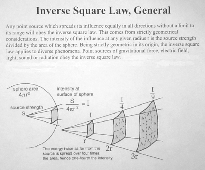

 

Before breaking down the equipment at the end of the lab, turn off the HV by clicking the button next to the voltage value. The positive HV light on the UCS-30 should turn green.  Place the \(^{60}\rm{Co}\) sample back into its plastic case and return it to the Lab Instructor.

Background Equipment Summary Questions