Part 1: Measuring Component Values

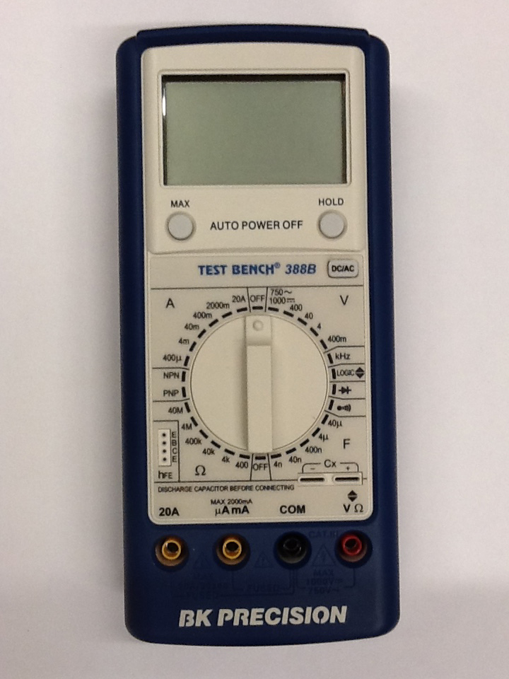
Remove the ohmic resistor that is attached to the white sheet of paper.  Use the BK DMM to measure its resistance (always make sure to record the meter range that you are using whenever you measure a value with a DMM). Calculate the value’s uncertainty.

Now remove the capacitor that is attached to the white sheet of paper.  Use the BK DMM to measure its capacitance (the capacitor is marked with a negative sign with an arrow pointing to the negative lead). Make sure that the capacitor is discharged before placing it in the meter.  Ask Lab Instructor for help if you do not know how to discharge the capacitor. Calculate the value’s uncertainty.

Calculate the circuit’s time constant \(\tau\) with uncertainty using the two measured values obtained above.

Part 2: Set up an RC Circuit

Set up an RC charging circuit using the batteries (make sure the three batteries are in series to produce approximately \(4.5\) \({\rm V}\) like last week), capacitor, and resistor.  Add the BK DMM to measure the voltage across the capacitor.  Draw the circuit in your notebook making sure to label all of its components.

Let the capacitor fully charge.  The voltage across the capacitor when it is fully charged is V Source.  Record V Source (without uncertainty) in your notebook.

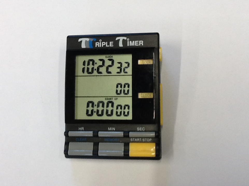
Using the timer and BK DMM, measure the voltage across the capacitor during the capacitor’s discharge cycle (make sure the capacitor is completely charged before starting).  Record both \(t\) and \(V\) starting at \(t=0\) \({\rm s}\) and ending at \(t=60\) \({\rm s}\).  Use a reasonable time interval that allows you and your partner to accurately record both \(t\) and \(V\).  The time interval should be as small as possible while still allowing for accurate measurements.  Calculate the uncertainty of one representative \(V\) value (one near the middle of the cycle).  Use your best estimate for \(\delta t\).

Plot \(V\) vs. \(t\).  Place error bars on the data point for which you determined  \(\delta V\) and \(\delta t\).

Use your plot to graphically determine the circuit’s time constant \(\tau\).  (Reminder: V at t=0 is Vo)

Now make sure the capacitor is fully discharged.  Using the timer and BK DMM, measure the voltage across the capacitor during the capacitor’s charging cycle.  Again record both \(t\) and \(V\) starting at \(t=0\) \({\rm s}\) and ending at \(t=60\) \({\rm s}\). Use the same reasonable time interval that you used above.  Calculate the uncertainty of one representative \(V\) value (one near the middle of the cycle).  Use your best estimate for \(\delta t\).

Plot \(V\) vs. \(t\).  Place error bars on the data point for which you determined  \(\delta V\) and \(\delta t\).

Use your plot to graphically determine the circuit’s time constant \(\tau\).

Part 3: Straight Line Analysis using Semi-Log Graph Paper

In 1130 Physics Lab we took non-linear data and made it linear thus allowing us to use straight line analysis to determine important characteristics of a system.  It is possible to plot our data as a straight line by using a special type of graph paper called semi-logarithmic (semi-log) graph paper.  Exponential functions plot as straight lines on semi-log graph paper.  Look at the sheet of semi-logarithmic graph paper that was provided to you.  Notice that the vertical scale is logarithmic while the horizontal scale is linear.

Exponential functions have the form:$$ y = k e^{mx} $$ or $$ \ln y = mx + \ln k$$

where \(m\) is any positive or negative constant.  Notice that the second equation is that of a line.  On semi-log graph paper \(m = {\rm the\;slope\;of\;the\;line}\) and \(k = {\rm the\;y-intercept}\).

Earlier we learned that the equation describing the discharge of a capacitor in series with a resistor is:$$ V(t) = V_{0}e^{-t/(RC)}$$                       

This is clearly an exponential function.  Now plot \(V\) vs. \(t\) on the semi-log graph paper using the data you collected when the capacitor was being discharged.  Note that you do not have to take the natural log of \(V\) before you plot it because the vertical scale is already logarithmic.  Draw the best fit line and calculate its slope* without uncertainty.

*Calculating the slope of a line plotted on semi-log graph paper is a little different than that of calculating the slope of a line plotted on linear graph paper. Because semi-log graph paper uses two different scales, linear and logarithmic, it is necessary to convert the data of one axis to match that of the other before calculating the slope.  The most common method is to convert the logarithmic axis data to linear data by taking its natural log.  Therefore you must first calculate the natural log of your two \(Y\) values before you use them to calculate \(\Delta Y\) in your slope equation.

Thus:                   $${\rm Slope} = \frac{\ln Y_{2} – \ln Y_{1}}{X_{2} -X_{1}}$$

Note that \(\ln Y_{2}-\ln Y_{1} = \ln (Y_{2}/Y_{1})\), therefore it is unit-less.

Compare the time constants calculated from your three plots with the one calculated with the measured \(R\) and \(C\) values.  Do they agree within reason (keeping in mind that we have not calculated the uncertainty in the graphically calculated values)? What do you think caused the largest error in your values calculated with the plots?

Background Equipment Summary Questions